11.2. Convolutional Neural Network
Also Known as CNN
Combination of:
Deep Neural Networks
Kernel Convolutions
With assumption, that input is image
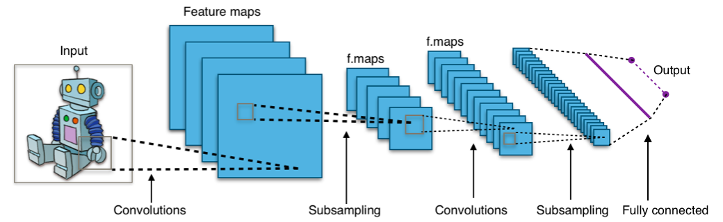
Figure 11.9. General overview of Convolutional Neural Network
11.2.1. Problemy z przetwarzaniem obrazów
cienie
nakładające się obrazy
zmiany kąta i pochyłości kamery
kąt padania światła
kolorystyka
zakrzywienia płaszczyzny
szumy
11.2.2. What is and Kernel Convolution?
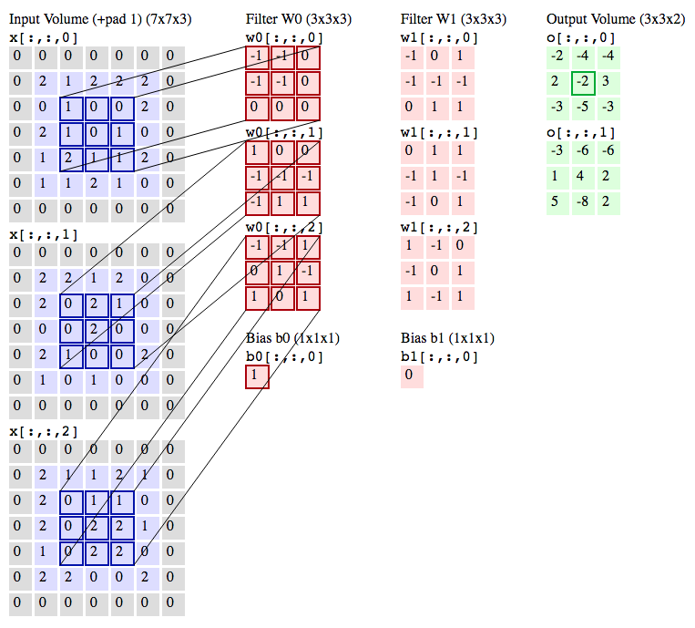
Figure 11.10. Convolutional Neural Network with 3x3 kernel convolutions

Figure 11.11. Convolution with 3x3 kernel for Mean Blur Filter
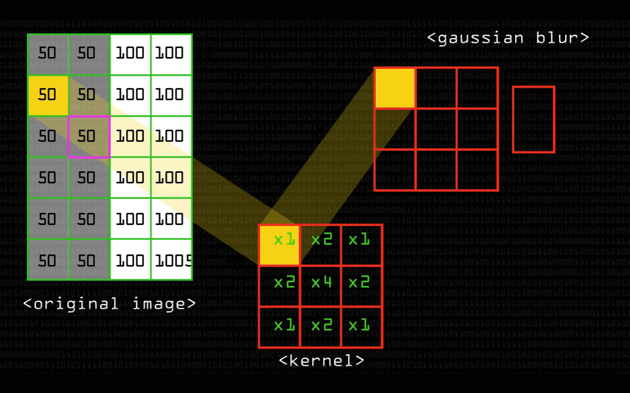
Figure 11.12. Convolution with 3x3 kernel for Gaussian Blur Filter
11.2.3. What is Convolutional Neural Network (CNN / ConvNet)
Figure 11.13. Architecture of the Convolutional Neural Network
Convolutional Neural Networks are very similar to ordinary Neural Networks from the previous chapter: they are made up of neurons that have learnable weights and biases. Each neuron receives some inputs, performs a dot product and optionally follows it with a non-linearity. The whole network still expresses a single differentiable score function: from the raw image pixels on one end to class scores at the other. And they still have a loss function (e.g. SVM/Softmax) on the last (fully-connected) layer and all the tips/tricks we developed for learning regular Neural Networks still apply.
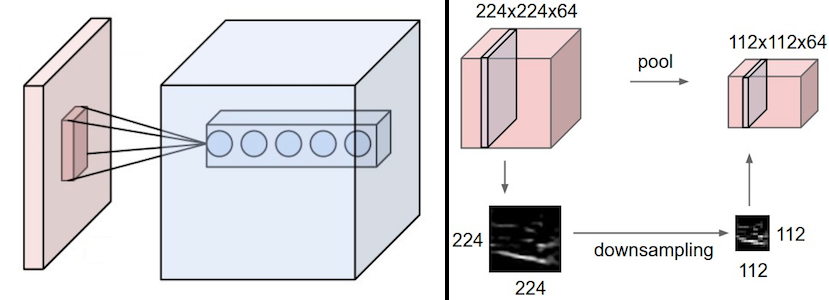
Figure 11.14. Convolutional Neural Network layer pool transformation
So what does change? ConvNet architectures make the explicit assumption that the inputs are images, which allows us to encode certain properties into the architecture. These then make the forward function more efficient to implement and vastly reduce the amount of parameters in the network.
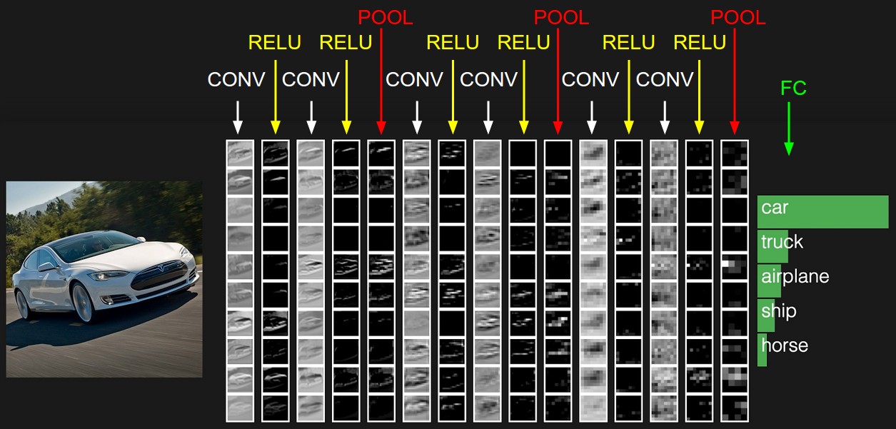
Figure 11.15. Convolutional Neural Network example
11.2.4. Handwritten digits recognition (MNIST) with sklearn
import matplotlib.pyplot as plt
from sklearn.datasets import fetch_mldata
from sklearn.neural_network import MLPClassifier


mnist = fetch_mldata("MNIST original")

# rescale the data, use the traditional train/test split
features = mnist.data / 255.
labels = mnist.target

features_train = features[:60000]
features_test = features[60000:]

labels_train = labels[:60000]
labels_test = labels[60000:]


model = MLPClassifier(
    hidden_layer_sizes=(50,),
    max_iter=10,
    alpha=1e-4,
    solver='sgd',
    verbose=10,
    tol=1e-4,
    random_state=1,
    learning_rate_init=.1
)

model.fit(features_train, labels_train)

training_score = model.score(features_train, labels_train)
test_score = model.score(features_test, labels_test)

print(f"Training set score: {training_score}")
print(f"Test set score: {test_score}")

fig, axes = plt.subplots(4, 4)

# use global min / max to ensure all weights are shown on the same scale
vmin = model.coefs_[0].min()
vmax = model.coefs_[0].max()


for coef, ax in zip(model.coefs_[0].T, axes.ravel()):

    # każdy obrazek to jest jeden neuron
    # Neuronów jest 50
    ax.matshow(
        coef.reshape(28, 28),
        cmap=plt.cm.gray,
        vmin=.5 * vmin,
        vmax=.5 * vmax)

    ax.set_xticks(())
    ax.set_yticks(())

plt.show()  # doctest: +SKIP
11.2.5. Handwritten digits recognition (MNIST) with tensorflow
import numpy as np
import tensorflow as tf

# Data sets
IRIS_TRAINING = '../_data/iris_training.csv'
IRIS_TEST = '../_data/iris_test.csv'


# Load datasets.
training_set = tf.contrib.learn.datasets.base.load_csv_with_header(
    filename=IRIS_TRAINING,
    target_dtype=np.int,
    features_dtype=np.float32)

test_set = tf.contrib.learn.datasets.base.load_csv_with_header(
    filename=IRIS_TEST,
    target_dtype=np.int,
    features_dtype=np.float32)


# Specify that all features have real-value data
feature_columns = [tf.contrib.layers.real_valued_column("", dimension=4)]


# Build 3 layer DNN with 10, 20, 10 units respectively.
classifier = tf.contrib.learn.DNNClassifier(
    feature_columns=feature_columns,
    hidden_units=[10, 20, 10],
    n_classes=3,
    model_dir="/tmp/iris_model")


# Define the training inputs
def get_train_inputs():
    x = tf.constant(training_set.data)
    y = tf.constant(training_set.target)
    return x, y


# Fit model.
classifier.fit(input_fn=get_train_inputs, steps=2000)


# Define the test inputs
def get_test_inputs():
    x = tf.constant(test_set.data)
    y = tf.constant(test_set.target)
    return x, y


# Evaluate accuracy.
accuracy_score = classifier.evaluate(input_fn=get_test_inputs, steps=1)["accuracy"]
print(f"\nTest Accuracy: {accuracy_score:f}\n")


# Classify two new flower samples.
def new_samples():
    return np.array(
        [[6.4, 3.2, 4.5, 1.5],
         [5.8, 3.1, 5.0, 1.7]], dtype=np.float32)


predictions = list(classifier.predict_classes(input_fn=new_samples))

print(f"New Samples, Class Predictions: {predictions}\n")

# Test Accuracy: 0.966667
# New Samples, Class Predictions: [1, 1]
11.2.6. Handwritten digits recognition (MNIST) with keras
Gets to 99.25% test accuracy after 12 epochs
import keras
from keras.datasets import mnist
from keras.models import Sequential
from keras.layers import Dense, Dropout, Flatten
from keras.layers import Conv2D, MaxPooling2D
from keras import backend as K

batch_size = 128
num_classes = 10
epochs = 12

# input image dimensions
img_rows, img_cols = 28, 28

# the data, shuffled and split between train and test sets
(x_train, y_train), (x_test, y_test) = mnist.load_data()

if K.image_data_format() == 'channels_first':
    x_train = x_train.reshape(x_train.shape[0], 1, img_rows, img_cols)
    x_test = x_test.reshape(x_test.shape[0], 1, img_rows, img_cols)
    input_shape = (1, img_rows, img_cols)
else:
    x_train = x_train.reshape(x_train.shape[0], img_rows, img_cols, 1)
    x_test = x_test.reshape(x_test.shape[0], img_rows, img_cols, 1)
    input_shape = (img_rows, img_cols, 1)

x_train = x_train.astype('float32')
x_test = x_test.astype('float32')
x_train /= 255
x_test /= 255
print('x_train shape:', x_train.shape)
print(x_train.shape[0], 'train samples')
print(x_test.shape[0], 'test samples')

# convert class vectors to binary class matrices
y_train = keras.utils.to_categorical(y_train, num_classes)
y_test = keras.utils.to_categorical(y_test, num_classes)

model = Sequential()
model.add(Conv2D(32, kernel_size=(3, 3),
                 activation='relu',
                 input_shape=input_shape))
model.add(Conv2D(64, (3, 3), activation='relu'))
model.add(MaxPooling2D(pool_size=(2, 2)))
model.add(Dropout(0.25))
model.add(Flatten())
model.add(Dense(128, activation='relu'))
model.add(Dropout(0.5))
model.add(Dense(num_classes, activation='softmax'))

model.compile(loss=keras.losses.categorical_crossentropy,
              optimizer=keras.optimizers.Adadelta(),
              metrics=['accuracy'])

model.fit(x_train, y_train,
          batch_size=batch_size,
          epochs=epochs,
          verbose=1,
          validation_data=(x_test, y_test))
score = model.evaluate(x_test, y_test, verbose=0)
print('Test loss:', score[0])
print('Test accuracy:', score[1])