9.1. Support Vector Machines

positive

negative

cluster

vector space

best separating hyperplane

classification

regression

generative model

decision boundary

discriminative model

distribution

Positive

Grupa zbioru

Negative

Grupa zbioru

Discriminative Classifier

Draws a boundary between clusters of data. For tasks such as classification and regression that do not require the joint distribution. discriminative model can yield superior performance over generative model.

Support Vector

Punkty które leżą na linii "marginesu"

Vector Space

Przestrzeń w której znajdują się dane. Dla danych (wektorów) dwuwymiarowych przestrzeń można zobrazować za pomocą wykresu 2D z kartezjańskim układem współrzędnych.

Binary classifier

Dzieli zbiór na dwie części positive i negative

Best separating hyperplane

Line that separates two decision boundary

9.1.1. TL;DR

• Jeden z najbardziej popularnych algorytmów Machine Learning

• Dzieli vector space za pomocą linii

• Wyszukuje linię taką linię, która ma największy margines pomiędzy wszystkimi punktami tzw. best separating hyperplane

• Dla nieznanego punktu sprawdza po której stronie krzywej się znajduje i na podstawie tego określa przynależność

• Linia prosta jest najprostszym przypadkiem

• Może się okazać, że konieczne będzie przeprowadzenie bardzo skomplikowanej krzywej

• Jeżeli dane są zgrupowane w wielowymiarowej przestrzeni, trzeba będzie użyć zbioru

9.1.2. Charakterystyka algorytmu

9.1.3. Przeznaczenie

9.1.4. Zalety algorytmu

• Guaranteed Optimality: Due to the nature of Convex Optimization, the solution is guaranteed to be the global minimum not a local minimum.

• Conformity with Semi-Supervised Learning: It may be used in a dataset where some of the data are labeled and some are not. You only add an additional condition to the minimization problem and it is called Transductive SVM.

• Feature Mapping might have been a burden on the computational complexity of the overall training performance; however, thanks to the 'Kernel Trick' the feature mapping is implicitly carried out via simple dot products.

9.1.5. Wady algorytmu

• In Natural Language Processing, structured representations of text yield better performances. Sadly, SVMs can not accommodate such structures(word embeddings) and are used through Bag-of-Words representation which loses sequentially information and leads to worse performance.

• SVM in its vanilla form cannot return a probabilistic confidence value like logistic regression does, in some sense it's not 'explanatory' enough.

9.1.6. Opis algorytmu

9.1.7. Definicja intuicyjna

U podstaw metody wektorów nośnych (Support Vector Machines - SVM) leży koncepcja przestrzeni decyzyjnej, którą dzieli się budując granice separujące obiekty o różnej przynależności klasowej, czego przykład widzimy na poniższym rysunku. Mamy tu dwie klasy kółek: czarne i białe. Linia graniczna rozdziela je wyraźnie. Nowy, nieznany obiekt, jeżeli znajdzie się po prawej stronie granicy zostanie zaklasyfikowany jako biały, a w przeciwnym wypadku, jako czarny.

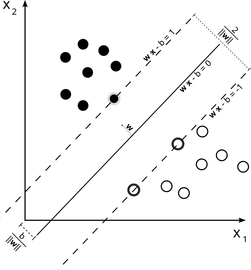
Figure 9.13. Maximum-margin hyperplane and margins for an SVM trained with samples from two classes. Samples on the margin are called the support vectors.

Powyższy rysunek jest ilustracją bardzo prostego przykładu klasyfikatora liniowego, dzielącego obszar prób na dwie części za pomocą prostej. Większość praktycznych zadań klasyfikacyjnych jednak nie jest tak oczywista. Do poprawnego klasyfikowania potrzebne są bardziej skomplikowane struktury niż linia prosta. Przykładem może być poniższy rysunek, który porównany z poprzednim jasno wskazuje, że do rozdzielenia kółek czarnych i białych konieczna jest teraz krzywa (obiekt bardziej skomplikowany niż prosta). Krzywa ta (ale również poprzednia prosta) są przykładami klasyfikatorów hiperpłaszczyznowych. Tego typu klasyfikatory otrzymujemy stosując Metodę wektorów nośnych.

9.1.8. Definicja formalna

• Tą metodą wykonuje się regresję i klasyfikację, konstruując nieliniowe granice decyzyjne.

• Istnieje kilka typów wektorów nośnych, z różnymi funkcjami bazowymi:

  • liniową, wielomianową,

  • RBF (radialne funkcje bazowe)

  • sigmoidalną.

9.1.9. Support Vector Machines (Kernels)

• \(f(x) = B0 + sum(ai * (x,xi))\)

• The equation for making a prediction for a new input using the dot product between the input (x) and each support vector (xi)

9.1.10. Linear Kernel SVM

• \(K(x, xi) = sum(x * xi)\)

The kernel defines the similarity or a distance measure between new data and the support vectors.

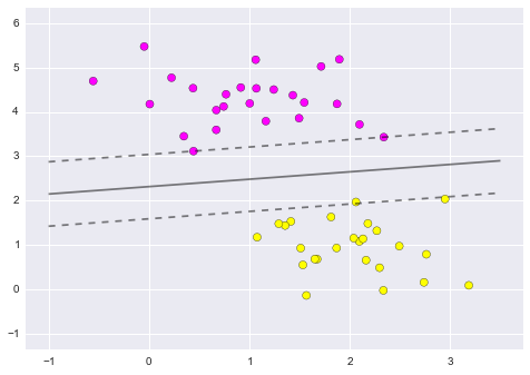
Figure 9.14. Linear Kernel SVM

9.1.11. Polynomial Kernel SVM

• \(K(x,xi) = 1 + sum(x * xi)^d\)

• Polynomial kernel

• Where the degree of the polynomial must be specified by hand to the learning algorithm.

• When \(d=1\) this is the same as the linear kernel.

• The polynomial kernel allows for curved lines in the input space.

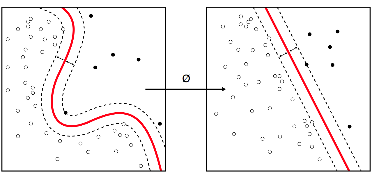
Figure 9.15. Polynomial Kernel SVM

9.1.12. Radial Kernel SVM

• \(K(x,xi) = exp(-gamma * sum((x – xi^2))\)

• Where gamma is a parameter that must be specified to the learning algorithm.

• A good default value for gamma is 0.1, where gamma is often 0 < gamma < 1.

• The radial kernel is very local and can create complex regions within the feature space, like closed polygons in two-dimensional space.

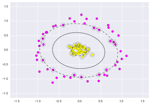
Figure 9.16. 2D Radial Kernel SVM

Figure 9.17. 3D Radial Kernel SVM

9.1.13. Przykłady praktyczne

9.1.14. Przykład wykorzystania sklearn

# import some data to play with
iris = datasets.load_iris()

# we only take the first two features: [:, :2]
X = iris.data[:, :2]
y = iris.target

from sklearn import svm

# Assumed you have, X (predictor) and Y (target) for training data set and x_test(predictor) of test_dataset
# Create SVM classification object
model = svm.SVC(kernel='linear', c=1, gamma=1)

# there is various option associated with it, like changing kernel, gamma and C value. Will discuss more # about it in next section.Train the model using the training sets and check score
model.fit(X, y)
model.score(X, y)

# Predict Output
predicted = model.predict(x_test)

9.1.15. Przygotowanie do przykładów

import numpy as np
import matplotlib.pyplot as plt
from scipy import stats

# use seaborn plotting defaults
import seaborn as sns

sns.set()

9.1.16. Motivating Support Vector Machines

Support Vector Machines (SVMs) are a powerful supervised learning algorithm used for classification or for regression. SVMs are a discriminative classifier: that is, they draw a boundary between clusters of data.

Let's show a quick example of support vector classification. First we need to create a dataset:

from sklearn.datasets.samples_generator import make_blobs
X, y = make_blobs(n_samples=50, centers=2,
                  random_state=0, cluster_std=0.60)
plt.scatter(X[:, 0], X[:, 1], c=y, s=50, cmap='spring');

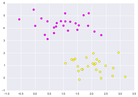
Figure 9.18. A discriminative classifier attempts to draw a line between the two sets of data.

A discriminative classifier attempts to draw a line between the two sets of data. Immediately we see a problem: such a line is ill-posed! For example, we could come up with several possibilities which perfectly discriminate between the classes in this example:

xfit = np.linspace(-1, 3.5)
plt.scatter(X[:, 0], X[:, 1], c=y, s=50, cmap='spring')

for m, b in [(1, 0.65), (0.5, 1.6), (-0.2, 2.9)]:
    plt.plot(xfit, m * xfit + b, '-k')

plt.xlim(-1, 3.5);

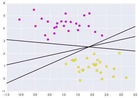
Figure 9.19. Depending on which you choose, a new data point will be classified almost entirely differently!

These are three very different separators which perfectly discriminate between these samples. Depending on which you choose, a new data point will be classified almost entirely differently!

How can we improve on this?

9.1.17. Maximizing the Margin

Support vector machines are one way to address this. What support vector machined do is to not only draw a line, but consider a region about the line of some given width. Here's an example of what it might look like:

xfit = np.linspace(-1, 3.5)
plt.scatter(X[:, 0], X[:, 1], c=y, s=50, cmap='spring')

for m, b, d in [(1, 0.65, 0.33), (0.5, 1.6, 0.55), (-0.2, 2.9, 0.2)]:
    yfit = m * xfit + b
    plt.plot(xfit, yfit, '-k')
    plt.fill_between(xfit, yfit - d, yfit + d, edgecolor='none', color='#AAAAAA', alpha=0.4)

plt.xlim(-1, 3.5);

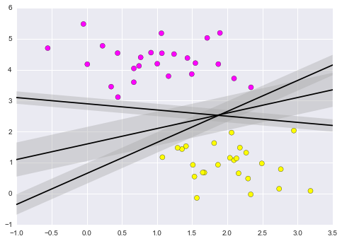
Figure 9.20. What support vector machined do is to not only draw a line, but consider a region about the line of some given width.

Notice here that if we want to maximize this width, the middle fit is clearly the best. This is the intuition of support vector machines, which optimize a linear discriminant model in conjunction with a margin representing the perpendicular distance between the datasets.

9.1.18. Fitting a Support Vector Machine

Now we'll fit a Support Vector Machine Classifier to these points. While the mathematical details of the likelihood model are interesting, we'll let you read about those elsewhere. Instead, we'll just treat the scikit-learn algorithm as a black box which accomplishes the above task.

from sklearn.svm import SVC # "Support Vector Classifier"

clf = SVC(kernel='linear')

clf.fit(X, y)
# SVC(C=1.0, cache_size=200, class_weight=None, coef0=0.0, degree=3, gamma=0.0,
#     kernel='linear', max_iter=-1, probability=False, random_state=None,
#     shrinking=True, tol=0.001, verbose=False)

To better visualize what's happening here, let's create a quick convenience function that will plot SVM decision boundaries for us:

def plot_svc_decision_function(clf, ax=None):
    """Plot the decision function for a 2D SVC"""

    if ax is None:
        ax = plt.gca()

    x = np.linspace(plt.xlim()[0], plt.xlim()[1], 30)
    y = np.linspace(plt.ylim()[0], plt.ylim()[1], 30)
    Y, X = np.meshgrid(y, x)
    P = np.zeros_like(X)

    for i, xi in enumerate(x):
        for j, yj in enumerate(y):
            P[i, j] = clf.decision_function([xi, yj])

    # plot the margins
    ax.contour(X, Y, P, colors='k',
               levels=[-1, 0, 1], alpha=0.5,
               linestyles=['--', '-', '--'])

plt.scatter(X[:, 0], X[:, 1], c=y, s=50, cmap='spring')
plot_svc_decision_function(clf);

Figure 9.21. Notice that the dashed lines touch a couple of the points: these points are the pivotal pieces of this fit, and are known as the support vectors (giving the algorithm its name).

Notice that the dashed lines touch a couple of the points: these points are the pivotal pieces of this fit, and are known as the support vectors (giving the algorithm its name). In scikit-learn, these are stored in the support_vectors_ attribute of the classifier:

plt.scatter(X[:, 0], X[:, 1], c=y, s=50, cmap='spring')
plot_svc_decision_function(clf)
plt.scatter(clf.support_vectors_[:, 0], clf.support_vectors_[:, 1],
            s=200, facecolors='none');

Figure 9.22. Support Vector Machines

Let's use IPython's interact functionality to explore how the distribution of points affects the support vectors and the discriminative fit. (This is only available in IPython 2.0+, and will not work in a static view)

from IPython.html.widgets import interact

def plot_svm(N=10):
    X, y = make_blobs(n_samples=200, centers=2,
                      random_state=0, cluster_std=0.60)
    X = X[:N]
    y = y[:N]

    clf = SVC(kernel='linear')
    clf.fit(X, y)

    plt.scatter(X[:, 0], X[:, 1], c=y, s=50, cmap='spring')
    plt.xlim(-1, 4)
    plt.ylim(-1, 6)

    plot_svc_decision_function(clf, plt.gca())
    plt.scatter(clf.support_vectors_[:, 0], clf.support_vectors_[:, 1],
                s=200, facecolors='none')

interact(plot_svm, N=[10, 200], kernel='linear');

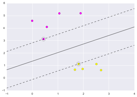
Figure 9.23. Notice the unique thing about SVM is that only the support vectors matter: that is, if you moved any of the other points without letting them cross the decision boundaries, they would have no effect on the classification results!

Notice the unique thing about SVM is that only the support vectors matter: that is, if you moved any of the other points without letting them cross the decision boundaries, they would have no effect on the classification results!

9.1.19. Going further: Kernel Methods

Where SVM gets incredibly exciting is when it is used in conjunction with kernels. To motivate the need for kernels, let's look at some data which is not linearly separable:

from sklearn.datasets.samples_generator import make_circles

X, y = make_circles(100, factor=.1, noise=.1)

clf = SVC(kernel='linear').fit(X, y)

plt.scatter(X[:, 0], X[:, 1], c=y, s=50, cmap='spring')
plot_svc_decision_function(clf);

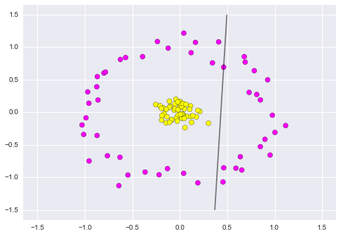
Figure 9.24. Clearly, no linear discrimination will ever separate these data.

Clearly, no linear discrimination will ever separate these data. One way we can adjust this is to apply a kernel, which is some functional transformation of the input data.

For example, one simple model we could use is a radial basis function

r = np.exp(-(X[:, 0] ** 2 + X[:, 1] ** 2))

If we plot this along with our data, we can see the effect of it:

from mpl_toolkits import mplot3d

def plot_3D(elev=30, azim=30):
    ax = plt.subplot(projection='3d')
    ax.scatter3D(X[:, 0], X[:, 1], r, c=y, s=50, cmap='spring')
    ax.view_init(elev=elev, azim=azim)
    ax.set_xlabel('x')
    ax.set_ylabel('y')
    ax.set_zlabel('r')

interact(plot_3D, elev=[-90, 90], azip=(-180, 180));

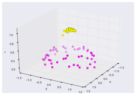
Figure 9.25. We can see that with this additional dimension, the data becomes trivially linearly separable!

We can see that with this additional dimension, the data becomes trivially linearly separable! This is a relatively simple kernel; SVM has a more sophisticated version of this kernel built-in to the process. This is accomplished by using kernel='rbf' , short for radial basis function:

clf = SVC(kernel='rbf')
clf.fit(X, y)

plt.scatter(X[:, 0], X[:, 1], c=y, s=50, cmap='spring')
plot_svc_decision_function(clf)
plt.scatter(clf.support_vectors_[:, 0], clf.support_vectors_[:, 1],
            s=200, facecolors='none');

Figure 9.26. Here there are effectively \(N\) basis functions: one centered at each point!

Here there are effectively \(N\) basis functions: one centered at each point! Through a clever mathematical trick, this computation proceeds very efficiently using the "Kernel Trick", without actually constructing the matrix of kernel evaluations.

We'll leave SVMs for the time being and take a look at another classification algorithm: Random Forests.

Source: https://github.com/jakevdp/sklearn_pycon2015/blob/master/notebooks/03.1-Classification-SVMs.ipynb

9.1.20. Assignments

9.1.20.1. Wykorzystanie biblioteki sklearn

• Assignment: Wykorzystanie biblioteki sklearn

• Complexity: medium

• Lines of code: 30 lines

• Time: 21 min

English:

TODO: English Translation X. Run doctests - all must succeed

Polish:

1. Naucz algorytm rozpoznawania danych wykorzystując algorytm Support Vector Machines.

2. Uruchom doctesty - wszystkie muszą się powieść

Given:

DATA = 'https://archive.ics.uci.edu/ml/machine-learning-databases/breast-cancer-wisconsin/'