8.2. Statistics

8.2.1. Mean

• Compute the arithmetic mean along the specified axis.

• The arithmetic mean is the sum of the elements along the axis divided by the number of elements.

• The average is taken over the flattened array by default, otherwise over the specified axis.

>>> import numpy as np

>>> a = np.array([1, 2, 3])
>>>
>>> np.mean(a)
2.0
>>>
>>> np.mean(a, axis=0)
2.0
>>>
>>> np.mean(a, axis=1)
Traceback (most recent call last):
numpy.exceptions.AxisError: axis 1 is out of bounds for array of dimension 1

>>> a = np.array([[1, 2, 3],
...               [4, 5, 6]])
>>>
>>> np.mean(a)
3.5
>>>
>>> np.mean(a, axis=0)
array([2.5, 3.5, 4.5])
>>>
>>> np.mean(a, axis=1)
array([2., 5.])

>>> a = np.array([[1, 2, 3],
...               [4, 5, 6],
...               [7, 8, 9]])
>>>
>>> np.mean(a)
5.0
>>>
>>> np.mean(a, axis=0)
array([4., 5., 6.])
>>>
>>> np.mean(a, axis=1)
array([2., 5., 8.])

8.2.2. Average

• Compute the weighted average along the specified axis.

>>> import numpy as np

>>> a = np.array([1, 2, 3])
>>>
>>> np.average(a)
2.0
>>>
>>> np.average(a, axis=0)
2.0
>>>
>>> np.average(a, axis=1)
Traceback (most recent call last):
numpy.exceptions.AxisError: axis 1 is out of bounds for array of dimension 1
>>>
>>> np.average(a, weights=[1, 1, 2])
2.25

>>> a = np.array([[1, 2, 3],
...               [4, 5, 6]])
>>>
>>> np.average(a)
3.5
>>>
>>> np.average(a, axis=0)
array([2.5, 3.5, 4.5])
>>>
>>> np.average(a, axis=1)
array([2., 5.])
>>>
>>> np.average(a, weights=[[1, 0, 2],
...                        [2, 0, 1]])
3.5

>>> a = np.array([[1, 2, 3],
...               [4, 5, 6],
...               [7, 8, 9]])
>>>
>>> np.average(a)
5.0
>>>
>>> np.average(a, axis=0)
array([4., 5., 6.])
>>>
>>> np.average(a, axis=1)
array([2., 5., 8.])
>>>
>>> np.average(a, weights=[[1, 0, 2],
...                        [2, 0, 1],
...                        [1./4, 1./2, 1./3]])
4.2

8.2.3. Median

• Compute the median along the specified axis

>>> import numpy as np

>>> a = np.array([1, 2, 3])
>>>
>>> np.median(a)
2.0
>>>
>>> np.median(a, axis=0)
2.0
>>>
>>> np.median(a, axis=1)
Traceback (most recent call last):
numpy.exceptions.AxisError: axis 1 is out of bounds for array of dimension 1

>>> a = np.array([[1, 2, 3],
...               [4, 5, 6]])
>>>
>>> np.median(a)
3.5
>>>
>>> np.median(a, axis=0)
array([2.5, 3.5, 4.5])
>>>
>>> np.median(a, axis=1)
array([2., 5.])

>>> a = np.array([[1, 2, 3],
...               [4, 5, 6],
...               [7, 8, 9]])
>>>
>>> np.median(a)
5.0
>>>
>>> np.median(a, axis=0)
array([4., 5., 6.])
>>>
>>> np.median(a, axis=1)
array([2., 5., 8.])

>>> a = np.array([1, 2, 3, 4])
>>>
>>> np.median(a)
2.5

8.2.4. Variance

• Compute the variance along the specified axis.

• Variance of the array elements is a measure of the spread of a distribution.

• The variance is the average of the squared deviations from the mean, i.e., var = mean(abs(x - x.mean())**2)

• The variance is computed for the flattened array by default, otherwise over the specified axis.

>>> import numpy as np

>>> a = np.array([1, 2, 3])
>>>
>>> np.var(a)
0.6666666666666666
>>>
>>> np.var(a, axis=0)
0.6666666666666666
>>>
>>> np.var(a, axis=1)
Traceback (most recent call last):
numpy.exceptions.AxisError: axis 1 is out of bounds for array of dimension 1

>>> a = np.array([[1, 2, 3],
...               [4, 5, 6]])
>>>
>>> np.var(a)
2.9166666666666665
>>>
>>> np.var(a, axis=0)
array([2.25, 2.25, 2.25])
>>>
>>> np.var(a, axis=1)
array([0.66666667, 0.66666667])

>>> a = np.array([[1, 2, 3],
...               [4, 5, 6],
...               [7, 8, 9]])
>>>
>>> np.var(a)
6.666666666666667
>>>
>>> np.var(a, axis=0)
array([6., 6., 6.])
>>>
>>> np.var(a, axis=1)
array([0.66666667, 0.66666667, 0.66666667])

8.2.5. Standard Deviation

• Compute the standard deviation along the specified axis.

• Standard deviation is a measure of the spread of a distribution, of the array elements.

• The standard deviation is the square root of the average of the squared deviations from the mean, i.e., std = sqrt(mean(abs(x - x.mean())**2))

• The standard deviation is computed for the flattened array by default, otherwise over the specified axis.

>>> import numpy as np

>>> a = np.array([1, 2, 3])
>>>
>>> np.std(a)
0.816496580927726
>>>
>>> np.std(a, axis=0)
0.816496580927726
>>>
>>> np.std(a, axis=1)
Traceback (most recent call last):
numpy.exceptions.AxisError: axis 1 is out of bounds for array of dimension 1

>>> a = np.array([[1, 2, 3],
...               [4, 5, 6]])
>>>
>>> np.std(a)
1.707825127659933
>>>
>>> np.std(a, axis=0)
array([1.5, 1.5, 1.5])
>>>
>>> np.std(a, axis=1)
array([0.81649658, 0.81649658])

>>> a = np.array([[1, 2, 3],
...               [4, 5, 6],
...               [7, 8, 9]])
>>>
>>> np.std(a)
2.581988897471611
>>>
>>> np.std(a, axis=0)
array([2.44948974, 2.44948974, 2.44948974])
>>>
>>> np.std(a, axis=1)
array([0.81649658, 0.81649658, 0.81649658])

8.2.6. Covariance

• Estimate a covariance matrix, given data and weights

• Covariance indicates the level to which two variables vary together

• ddof - Delta Degrees of Freedom

>>> import numpy as np

>>> a = np.array([1, 2, 3])
>>>
>>> np.cov(a)
array(1.)
>>>
>>> np.cov(a, ddof=0)
array(0.66666667)
>>>
>>> np.cov(a, ddof=1)
array(1.)

>>> a = np.array([[1, 2, 3],
...               [4, 5, 6]])
>>>
>>> np.cov(a)
array([[1., 1.],
       [1., 1.]])
>>>
>>> np.cov(a, ddof=0)
array([[0.66666667, 0.66666667],
       [0.66666667, 0.66666667]])
>>>
>>> np.cov(a, ddof=1)
array([[1., 1.],
       [1., 1.]])

>>> a = np.array([[1, 2, 3],
...               [4, 5, 6],
...               [7, 8, 9]])
>>>
>>> np.cov(a)
array([[1., 1., 1.],
       [1., 1., 1.],
       [1., 1., 1.]])
>>>
>>> np.cov(a, ddof=0)
array([[0.66666667, 0.66666667, 0.66666667],
       [0.66666667, 0.66666667, 0.66666667],
       [0.66666667, 0.66666667, 0.66666667]])
>>>
>>> np.cov(a, ddof=1)
array([[1., 1., 1.],
       [1., 1., 1.],
       [1., 1., 1.]])

8.2.7. Correlation coefficient

• measure of the linear correlation between two variables X and Y

• Pearson correlation coefficient (PCC)

• Pearson product-moment correlation coefficient (PPMCC)

• bivariate correlation

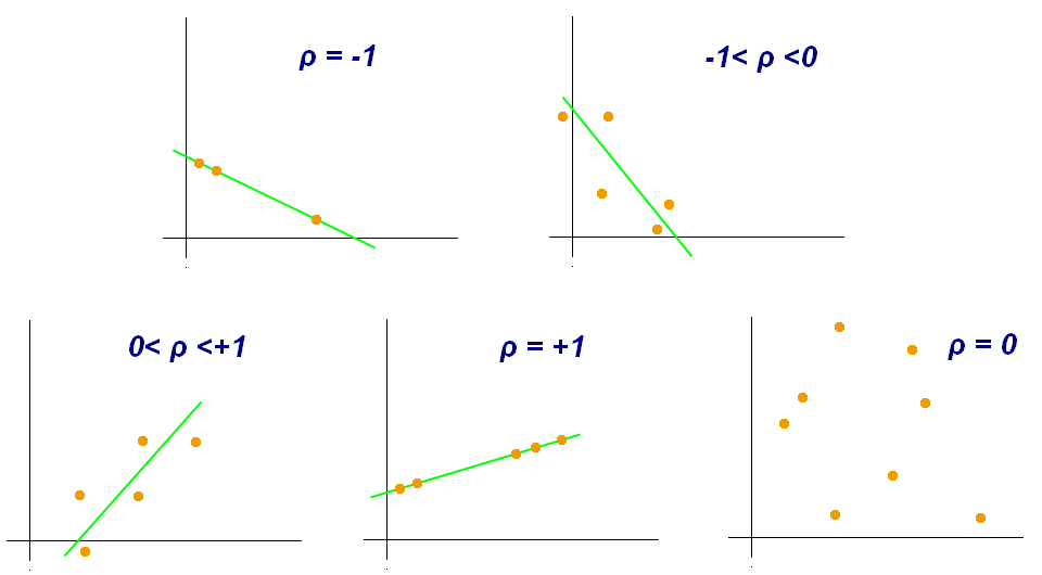
Figure 8.10. Examples of scatter diagrams with different values of correlation coefficient (ρ) [#NumpyPearsonCorrelationCoefficient]_

>>> import numpy as np

>>> a = np.array([1, 2, 3])
>>>
>>> np.corrcoef(a)
1.0

>>> a = np.array([[1, 2, 3],
...               [4, 5, 6]])
>>>
>>> np.corrcoef(a)
array([[1., 1.],
       [1., 1.]])

>>> a = np.array([[1, 2, 3],
...               [4, 5, 6],
...               [7, 8, 9]])
>>>
>>> np.corrcoef(a)
array([[1., 1., 1.],
       [1., 1., 1.],
       [1., 1., 1.]])

>>> a = np.array([[1, 2, 1],
...               [5, 4, 3]])
>>>
>>> np.corrcoef(a)
array([[1., 0.],
       [0., 1.]])

>>> a = np.array([[3, 1, 3],
...               [5, 5, 3]])
>>>
>>> np.corrcoef(a)
array([[ 1. , -0.5],
       [-0.5,  1. ]])

>>> a = np.array([[5, 2, 1],
...               [2, 4, 5]])
>>>
>>> np.corrcoef(a)
array([[ 1.        , -0.99587059],
       [-0.99587059,  1.        ]])

8.2.8. References

[1]

Wikipedia. Pearson correlation coefficient. Year: 2019. Retrieved: 2019-10-22. URL: https://en.wikipedia.org/wiki/Pearson_correlation_coefficient

[2]

Wikipedia. Normal distribution. Year: 2019. Retrieved: 2019-10-22. URL: https://en.wikipedia.org/wiki/Normal_distribution

[3]

Wikipedia. Poisson distribution. Year: 2019. Retrieved: 2019-10-22. URL: https://en.wikipedia.org/wiki/Poisson_distribution

[4]

Wikipedia. Continuous Uniform Distribution. Year: 2020. Retrieved: 2020-08-17. URL: https://en.wikipedia.org/wiki/Uniform_distribution_(continuous)

[5]

Wikipedia. Polynomial. Year: 2019. Retrieved: 2019-10-22. URL: https://en.wikipedia.org/wiki/Polynomial

[6]

Alex Chabot-Leclerc. Introduction to Numerical Computing with NumPy: Broadcasting Rules. Year: 2019. Retrieved: 2019-11-31. URL: https://youtu.be/ZB7BZMhfPgk?t=5142

[7]

Alex Chabot-Leclerc. Introduction to Numerical Computing with NumPy: Visualizing Multi-Dimensional Arrays. Year: 2019. Retrieved: 2019-12-05. URL: https://youtu.be/ZB7BZMhfPgk?t=5142