2.2. Basic Statistics
2.2.1. Rozkłady
kształty przebiegów
nazwy
zakresy
nadzieje
siły
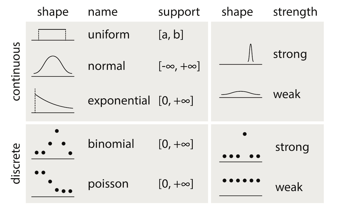
Figure 2.26. Rozkłady statystyczne
2.2.2. Podstawowe pojęcia
- Auto-regression Time Series
Value of the current time depends on the value of previous times.
- Funkcja
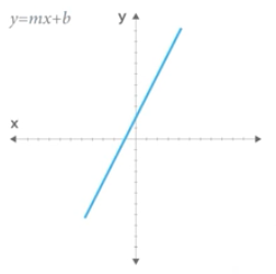
Figure 2.27. Funkcja opisana równaniem prostej \(f(x) = mx + b\)
- Równanie prostej
\(f(x) = ax + b\) lub \(f(x) = mx + b\)
- Models
Prototype for or the the rules that defines a body of classifier function. Typically models have parameters that allows to adjust the data. We use the training data to adjust the parameters of a model.
- Standard Deviation
Average distance from the mean for all the points.
- Average
A sometimes vague term. It usually denotes the arithmetic mean, but it can also denote the median, the mode, the geometric mean, and weighted means, among other things.
- Bayes' Rule
Bayes' rule expresses the conditional probability of the event \(A\) given the event \(B\) in terms of the conditional probability of the event \(B\) given the event \(A\) and the unconditional probability of \(A\):
\[P(A|B) = P(B|A) ×P(A)/( P(B|A)×P(A) + P(B|Ac) ×P(Ac) )\]In this expression, the unconditional probability of \(A\) is also called the prior probability of \(A\) , because it is the probability assigned to A prior to observing any data. Similarly, in this context, \(P(A|B)\) is called the posterior probability of \(A\) given \(B\) , because it is the probability of \(A\) updated to reflect (i.e., to condition on) the fact that \(B\) was observed to occur.
- Bernoulli's Inequality
The Bernoulli Inequality says that \(if x ≥ −1\) then \((1+x)n ≥ 1 + nx\) for every integer \(n ≥ 0\). If \(n\) is even, the inequality holds for all \(x\) .
- Chance variation, chance error
A random variable can be decomposed into a sum of its expected value and chance variation around its expected value. The expected value of the chance variation is zero; the standard error of the chance variation is the same as the standard error of the random variable—the size of a "typical" difference between the random variable and its expected value. See also sampling error.
- Class Boundary
A point that is the left endpoint of one class interval, and the right endpoint of another class interval.
- Class Interval
In plotting a histogram, one starts by dividing the range of values into a set of non-overlapping intervals, called class intervals, in such a way that every datum is contained in some class interval. See the related entries class boundary and endpoint convention.
- Cluster Sample
In a cluster sample, the sampling unit is a collection of population units, not single population units. For example, techniques for adjusting the U.S. census start with a sample of geographic blocks, then (try to) enumerate all inhabitants of the blocks in the sample to obtain a sample of people. This is an example of a cluster sample. (The blocks are chosen separately from different strata, so the overall design is a stratified cluster sample.)
- Conditional Probability
Suppose we are interested in the probability that some event \(A\) occurs, and we learn that the event \(B\) occurred. How should we update the probability of \(A\) to reflect this new knowledge? This is what the conditional probability does: it says how the additional knowledge that \(B\) occurred should affect the probability that \(A\) occurred quantitatively.
For example, suppose that \(A\) and \(B\) are mutually exclusive. Then if \(B\) occurred, \(A\) did not, so the conditional probability that \(A\) occurred given that \(B\) occurred is zero. At the other extreme, suppose that \(B\) is a subset of \(A\) , so that \(A\) must occur whenever \(B\) does. Then if we learn that \(B\) occurred, \(A\) must have occurred too, so the conditional probability that \(A\) occurred given that \(B\) occurred is 100%. For in-between cases, where \(A\) and \(B\) intersect, but \(B\) is not a subset of \(A\) , the conditional probability of \(A\) given \(B\) is a number between zero and 100%. Basically, one "restricts" the outcome space \(S\) to consider only the part of \(S\) that is in \(B\) , because we know that \(B\) occurred. For \(A\) to have happened given that \(B\) happened requires that \(AB\) happened, so we are interested in the event \(AB\) . To have a legitimate probability requires that \(P(S) = 100\%\) , so if we are restricting the outcome space to \(B\) , we need to divide by the probability of \(B\) to make the probability of this new \(S\) be 100%. On this scale, the probability that \(AB\) happened is \(P(AB)/P(B)\). This is the definition of the conditional probability of \(A\) given \(B\) , provided \(P(B)\) is not zero (division by zero is undefined). Note that the special cases \(AB = {}\) (\(A\) and \(B\) are mutually exclusive) and \(AB = B\) (\(B\) is a subset of \(A\)) agree with our intuition as described at the top of this paragraph. Conditional probabilities satisfy the axioms of probability, just as ordinary probabilities do.
- Converse
If \(p\) and \(q\) are two logical propositions, then the converse of the proposition \((p → q)\) is the proposition \((q → p)\) .
- Correlation
A measure of linear association between two (ordered) lists. Two variables can be strongly correlated without having any causal relationship, and two variables can have a causal relationship and yet be uncorrelated.
- Correlation coefficient
The correlation coefficient \(r\) is a measure of how nearly a scatterplot falls on a straight line. The correlation coefficient is always between −1 and +1. To compute the correlation coefficient of a list of pairs of measurements \((X,Y)\), first transform \(X\) and \(Y\) individually into standard units. Multiply corresponding elements of the transformed pairs to get a single list of numbers. The correlation coefficient is the mean of that list of products. This page contains a tool that lets you generate bivariate data with any correlation coefficient you want.
- Deviation
A deviation is the difference between a datum and some reference value, typically the mean of the data. In computing the SD, one finds the rms of the deviations from the mean, the differences between the individual data and the mean of the data.
- Discrete Variable
A quantitative variable whose set of possible values is countable. Typical examples of discrete variables are variables whose possible values are a subset of the integers, such as Social Security numbers, the number of people in a family, ages rounded to the nearest year, etc. Discrete variables are "chunky." C.f. continuous variable. A discrete random variable is one whose set of possible values is countable. A random variable is discrete if and only if its cumulative probability distribution function is a stair-step function; i.e., if it is piecewise constant and only increases by jumps.
- Distribution
The distribution of a set of numerical data is how their values are distributed over the real numbers. It is completely characterized by the empirical distribution function. Similarly, the probability distribution of a random variable is completely characterized by its probability distribution function. Sometimes the word "distribution" is used as a synonym for the empirical distribution function or the probability distribution function. If two or more random variables are defined for the same experiment, they have a joint probability distribution.
- Distribution Function, Empirical
The empirical (cumulative) distribution function of a set of numerical data is, for each real value of \(x\) , the fraction of observations that are less than or equal to \(x\) . A plot of the empirical distribution function is an uneven set of stairs. The width of the stairs is the spacing between adjacent data; the height of the stairs depends on how many data have exactly the same value. The distribution function is zero for small enough (negative) values of \(x\) , and is unity for large enough values of \(x\) . It increases monotonically: \(if y > x\), the empirical distribution function evaluated at \(y\) is at least as large as the empirical distribution function evaluated at \(x\).
- Expectation, Expected Value
The expected value of a random variable is the long-term limiting average of its values in independent repeated experiments. The expected value of the random variable \(X\) is denoted \(EX\) or \(E(X)\) . For a discrete random variable (one that has a countable number of possible values) the expected value is the weighted average of its possible values, where the weight assigned to each possible value is the chance that the random variable takes that value. One can think of the expected value of a random variable as the point at which its probability histogram would balance, if it were cut out of a uniform material. Taking the expected value is a linear operation: if \(X\) and \(Y\) are two random variables, the expected value of their sum is the sum of their expected values \((E(X+Y) = E(X) + E(Y))\) , and the expected value of a constant a times a random variable \(X\) is the constant times the expected value of \(X\) \((E(a×X ) = a× E(X))\) .
- Extrapolation
See interpolation.
- Game Theory
A field of study that bridges mathematics, statistics, economics, and psychology. It is used to study economic behavior, and to model conflict between nations, for example, "nuclear stalemate" during the Cold War.
- Geometric Distribution
The geometric distribution describes the number of trials up to and including the first success, in independent trials with the same probability of success. The geometric distribution depends only on the single parameter p, the probability of success in each trial. For example, the number of times one must toss a fair coin until the first time the coin lands heads has a geometric distribution with parameter \(p = 50\%\) . The geometric distribution assigns probability \(p×(1 − p)k−1\) to the event that it takes k trials to the first success. The expected value of the geometric distribution is \(1/p\) , and its SE is \((1−p)½/p\).
- Geometric Mean
The geometric mean of n numbers \({x1, x2, x3, ..., xn}\) is the nth root of their product:
\((x1×x2×x3× ... ×xn)1/n\)
- Histogram
A histogram is a kind of plot that summarizes how data are distributed. Starting with a set of class intervals, the histogram is a set of rectangles ("bins") sitting on the horizontal axis. The bases of the rectangles are the class intervals, and their heights are such that their areas are proportional to the fraction of observations in the corresponding class intervals. That is, the height of a given rectangle is the fraction of observations in the corresponding class interval, divided by the length of the corresponding class interval. A histogram does not need a vertical scale, because the total area of the histogram must equal 100%. The units of the vertical axis are percent per unit of the horizontal axis. This is called the density scale. The horizontal axis of a histogram needs a scale. If any observations coincide with the endpoints of class intervals, the endpoint convention is important. This page contains a histogram tool, with controls to highlight ranges of values and read their areas.
- Interpolation
Given a set of bivariate data \((x, y)\), to impute a value of \(y\) corresponding to some value of \(x\) at which there is no measurement of \(y\) is called interpolation, if the value of \(x\) is within the range of the measured values of \(x\) . If the value of \(x\) is outside the range of measured values, imputing a corresponding value of \(y\) is called extrapolation.
- Linear association
Two variables are linearly associated if a change in one is associated with a proportional change in the other, with the same constant of proportionality throughout the range of measurement. The correlation coefficient measures the degree of linear association on a scale of −1 to 1.
- Mean, Arithmetic mean
The sum of a list of numbers, divided by the number of elements in the list. See also average.
- Median
"Middle value" of a list. The smallest number such that at least half the numbers in the list are no greater than it. If the list has an odd number of entries, the median is the middle entry in the list after sorting the list into increasing order. If the list has an even number of entries, the median is the smaller of the two middle numbers after sorting. The median can be estimated from a histogram by finding the smallest number such that the area under the histogram to the left of that number is 50%.
- Member of a set
Something is a member (or element) of a set if it is one of the things in the set.
- Nonlinear Association
The relationship between two variables is nonlinear if a change in one is associated with a change in the other that is depends on the value of the first; that is, if the change in the second is not simply proportional to the change in the first, independent of the value of the first variable.
- Normal approximation
The normal approximation to data is to approximate areas under the histogram of data, transformed into standard units, by the corresponding areas under the normal curve.
Many probability distributions can be approximated by a normal distribution, in the sense that the area under the probability histogram is close to the area under a corresponding part of the normal curve. To find the corresponding part of the normal curve, the range must be converted to standard units, by subtracting the expected value and dividing by the standard error. For example, the area under the binomial probability histogram for \(n = 50\) and \(p = 30\%\) between 9.5 and 17.5 is 74.2%. To use the normal approximation, we transform the endpoints to standard units, by subtracting the expected value (for the Binomial random variable, \(n×p = 15\) for these values of \(n\) and \(p\) ) and dividing the result by the standard error (for a Binomial, \((n × p × (1−p))1/2 = 3.24\) for these values of \(n\) and \(p\)). The area normal approximation is the area under the normal curve between \((9.5 − 15)/3.24 = −1.697\) and \((17.5 − 15)/3.24 = 0.772\) ; that area is 73.5%, slightly smaller than the corresponding area under the binomial histogram. See also the continuity correction. The tool on this page illustrates the normal approximation to the binomial probability histogram. Note that the approximation gets worse when p gets close to 0 or 1, and that the approximation improves as n increases.
- Normal curve
The normal curve is the familiar "bell curve:," illustrated on this page. The mathematical expression for the normal curve is y = \((2×pi)−½e−x2/2\), where pi is the ratio of the circumference of a circle to its diameter (3.14159265...), and e is the base of the natural logarithm (2.71828...). The normal curve is symmetric around the point \(x=0\) , and positive for every value of \(x\). The area under the normal curve is unity, and the SD of the normal curve, suitably defined, is also unity. Many (but not most) histograms, converted into standard units, approximately follow the normal curve.
- Normal distribution
A random variable \(X\) has a normal distribution with mean \(m\) and standard error s if for every pair of numbers \(a ≤ b\), the chance that \(a < (X−m)/s < b\) is
\(P(a < (X−m)/s < b)\) = area under the normal curve between \(a\) and \(b\) .
If there are numbers m and s such that \(X\) has a normal distribution with mean m and standard error \(s\) , then \(X\) is said to have a normal distribution or to be normally distributed. If \(X\) has a normal distribution with mean \(m=0\) and standard error \(s=1\) , then \(X\) is said to have a standard normal distribution. The notation \(X~N(m,s2)\) means that \(X\) has a normal distribution with mean \(m\) and standard error \(s\) ; for example, \(X~N(0,1)\) , means \(X\) has a standard normal distribution.
- Partition
A partition of an event \(A\) is a collection of events \({A1, A2, A3, ... }\) such that the events in the collection are disjoint, and their union is \(A\). That is, \(AjAk = {}\) unless \(j = k\) , and \(A = A1 ∪ A2 ∪ A3 ∪ ...\) .
If the event \(A\) is not specified, it is assumed to be the entire outcome space \(S\) .
- Percentile
The pth percentile of a list is the smallest number such that at least \(p\%\) of the numbers in the list are no larger than it. The \(pth\) percentile of a random variable is the smallest number such that the chance that the random variable is no larger than it is at least \(p\%\) . C.f. quantile.
- Population
A collection of units being studied. Units can be people, places, objects, epochs, drugs, procedures, or many other things. Much of statistics is concerned with estimating numerical properties (parameters) of an entire population from a random sample of units from the population.
- Population Mean
The mean of the numbers in a numerical population. For example, the population mean of a box of numbered tickets is the mean of the list comprised of all the numbers on all the tickets. The population mean is a parameter. C.f. sample mean.
- Population Standard Deviation
The standard deviation of the values of a variable for a population. This is a parameter, not a statistic. C.f. sample standard deviation.
- Probability
The probability of an event is a number between zero and 100%. The meaning (interpretation) of probability is the subject of theories of probability, which differ in their interpretations. However, any rule for assigning probabilities to events has to satisfy the axioms of probability.
- Probability density function
The chance that a continuous random variable is in any range of values can be calculated as the area under a curve over that range of values. The curve is the probability density function of the random variable. That is, if \(X\) is a continuous random variable, there is a function \(f(x)\) such that for every pair of numbers a≤b,
\(P(a≤ X ≤b)\) = (area under \(f\) between \(a\) and \(b\) );
\(f\) is the probability density function of \(X\) . For example, the probability density function of a random variable with a standard normal distribution is the normal curve. Only continuous random variables have probability density functions.
- Probability Distribution
The probability distribution of a random variable specifies the chance that the variable takes a value in any subset of the real numbers. (The subsets have to satisfy some technical conditions that are not important for this course.) The probability distribution of a random variable is completely characterized by the cumulative probability distribution function; the terms sometimes are used synonymously. The probability distribution of a discrete random variable can be characterized by the chance that the random variable takes each of its possible values. For example, the probability distribution of the total number of spots \(S\) showing on the roll of two fair dice can be written as a table:
\(s\)
\(P(S=s)\)
2
1/36
3
2/36
4
3/36
5
4/36
6
5/36
7
6/36
8
5/36
9
4/36
10
3/36
11
2/36
12
1/36
The probability distribution of a continuous random variable can be characterized by its probability density function.
- Probability Histogram
A probability histogram for a random variable is analogous to a histogram of data, but instead of plotting the area of the bins proportional to the relative frequency of observations in the class interval, one plots the area of the bins proportional to the probability that the random variable is in the class interval.
- Quantile
The \(qth\) quantile of a list \((0 < q ≤ 1)\) is the smallest number such that the fraction q or more of the elements of the list are less than or equal to it. I.e., if the list contains \(n\) numbers, the \(qth\) quantile, is the smallest number \(Q\) such that at least \(n×q\) elements of the list are less than or equal to \(Q\).
- Random Sample
A random sample is a sample whose members are chosen at random from a given population in such a way that the chance of obtaining any particular sample can be computed. The number of units in the sample is called the sample size, often denoted \(n\) . The number of units in the population often is denoted \(N\). Random samples can be drawn with or without replacing objects between draws; that is, drawing all \(n\) objects in the sample at once (a random sample without replacement), or drawing the objects one at a time, replacing them in the population between draws (a random sample with replacement). In a random sample with replacement, any given member of the population can occur in the sample more than once. In a random sample without replacement, any given member of the population can be in the sample at most once. A random sample without replacement in which every subset of \(n\) of the \(N\) units in the population is equally likely is also called a simple random sample. The term random sample with replacement denotes a random sample drawn in such a way that every multiset of \(n\) units in the population is equally likely. See also probability sample.
- Random Variable
A random variable is an assignment of numbers to possible outcomes of a random experiment. For example, consider tossing three coins. The number of heads showing when the coins land is a random variable: it assigns the number 0 to the outcome \({T, T, T}\), the number 1 to the outcome \({T, T, H}\), the number 2 to the outcome \({T, H, H}\), and the number 3 to the outcome \({H, H, H}\).
- Real number
Loosely speaking, the real numbers are all numbers that can be represented as fractions (rational numbers), whether proper or improper—and all numbers in between the rational numbers. That is, the real numbers comprise the rational numbers and all limits of Cauchy sequences of rational numbers, where the Cauchy sequence is with respect to the absolute value metric. (More formally, the real numbers are the completion of the set of rational numbers in the topology induced by the absolute value function.) The real numbers contain all integers, all fractions, and all irrational (and transcendental) numbers, such as \(\pi\), \(e\) , and \(2½\). There are uncountably many real numbers between 0 and 1; in contrast, there are only countably many rational numbers between 0 and 1.
- Regression, Linear Regression
Linear regression fits a line to a scatterplot in such a way as to minimize the sum of the squares of the residuals. The resulting regression line, together with the standard deviations of the two variables or their correlation coefficient, can be a reasonable summary of a scatterplot if the scatterplot is roughly football-shaped. In other cases, it is a poor summary. If we are regressing the variable \(Y\) on the variable \(X\) , and if \(Y\) is plotted on the vertical axis and \(X\) is plotted on the horizontal axis, the regression line passes through the point of averages, and has slope equal to the correlation coefficient times the SD of \(Y\) divided by the SD of \(X\). This page shows a scatterplot, with a button to plot the regression line.
- Sample
A sample is a collection of units from a population. See also random sample.
- Sample Mean
The arithmetic mean of a random sample from a population. It is a statistic commonly used to estimate the population mean. Suppose there are \(n\) data, \({x1, x2, ... , xn}\). The sample mean is \((x1 + x2 + ... + xn)/n\) . The expected value of the sample mean is the population mean. For sampling with replacement, the SE of the sample mean is the population standard deviation, divided by the square-root of the sample size. For sampling without replacement, the SE of the sample mean is the finite-population correction \(((N−n)/(N−1))½\) times the SE of the sample mean for sampling with replacement, with \(N\) the size of the population and n the size of the sample.
- Standard Deviation (SD)
The standard deviation of a set of numbers is the rms of the set of deviations between each element of the set and the mean of the set. See also sample standard deviation.
- Standard Error (SE)
The Standard Error of a random variable is a measure of how far it is likely to be from its expected value; that is, its scatter in repeated experiments. The SE of a random variable \(X\) is defined to be
\[SE(X) = [E( (X − E(X))2 )] ½.\]That is, the standard error is the square-root of the expected squared difference between the random variable and its expected value. The SE of a random variable is analogous to the SD of a list.
- Standard Normal Curve
See normal curve.
- Transformation
Transformations turn lists into other lists, or variables into other variables. For example, to transform a list of temperatures in degrees Celsius into the corresponding list of temperatures in degrees Fahrenheit, you multiply each element by \(9/5\), and add 32 to each product. This is an example of an affine transformation: multiply by something and add something (\(y = ax + b\) is the general affine transformation of \(x\) ; it's the familiar equation of a straight line). In a linear transformation, you only multiply by something (\(y = ax\) ). Affine transformations are used to put variables in standard units. In that case, you subtract the mean and divide the results by the SD. This is equivalent to multiplying by the reciprocal of the SD and adding the negative of the mean, divided by the SD, so it is an affine transformation. Affine transformations with positive multiplicative constants have a simple effect on the mean, median, mode, quartiles, and other percentiles: the new value of any of these is the old one, transformed using exactly the same formula. When the multiplicative constant is negative, the mean, median, mode, are still transformed by the same rule, but quartiles and percentiles are reversed: the \(qth\) quantile of the transformed distribution is the transformed value of the \(1−qth\) quantile of the original distribution (ignoring the effect of data spacing). The effect of an affine transformation on the SD, range, and IQR, is to make the new value the old value times the absolute value of the number you multiplied the first list by: what you added does not affect them.
- Variable
A numerical value or a characteristic that can differ from individual to individual. See also categorical variable, qualitative variable, quantitative variable, discrete variable, continuous variable, and random variable.
- Variance, population variance
The variance of a list is the square of the standard deviation of the list, that is, the average of the squares of the deviations of the numbers in the list from their mean. The variance of a random variable \(X\) , \(Var(X)\) , is the expected value of the squared difference between the variable and its expected value: \(Var(X) = E((X − E(X))2)\) . The variance of a random variable is the square of the standard error (SE) of the variable.
- Venn Diagram
A pictorial way of showing the relations among sets or events. The universal set or outcome space is usually drawn as a rectangle; sets are regions within the rectangle. The overlap of the regions corresponds to the intersection of the sets. If the regions do not overlap, the sets are disjoint. The part of the rectangle included in one or more of the regions corresponds to the union of the sets. This page contains a tool that illustrates Venn diagrams; the tool represents the probability of an event by the area of the event.
Source: https://www.stat.berkeley.edu/~stark/SticiGui/Text/gloss.htm